Basic Usage Tutorial

This tutorial will walk you through the basic workflow of using Neurodent for rodent EEG analysis.

Overview

Neurodent provides a streamlined workflow for:

1. Loading EEG recordings from various formats

2. Extracting features from continuous data (Windowed Analysis)

3. Visualizing and analyzing results

Let’s get started!

1. Installation and Setup

First, ensure you have Neurodent installed. See the Installation Guide for detailed instructions.

pip install neurodent

Or with uv:

uv init yourprojectname
cd yourprojectname
uv add neurodent

2. Import Required Modules

Let’s import the necessary modules from Neurodent:

Tip: To see detailed progress information during processing, check out the Configuration Guide to learn how to enable logging.

from pathlib import Path
from datetime import datetime

import matplotlib.pyplot as plt

from neurodent import core, visualization, constants

/home/runner/work/neurodent/neurodent/.venv/lib/python3.10/site-packages/tqdm/auto.py:21: TqdmWarning: IProgress not found. Please update jupyter and ipywidgets. See https://ipywidgets.readthedocs.io/en/stable/user_install.html
  from .autonotebook import tqdm as notebook_tqdm

3. Configure Temporary Directory (Optional)

Neurodent uses a temporary directory for intermediate files during processing. You can set this to a location with sufficient space:

# Set temporary directory for intermediate files
# core.set_temp_directory("/path/to/your/temp/dir")

# Or use the default temp directory
print(f"Using temp directory: {core.get_temp_directory()}")

Using temp directory: /tmp

4. Load EEG Data

Neurodent supports multiple data formats through LongRecordingOrganizer (LRO):

• SpikeInterface mode (mode="si"): Load any format supported by SpikeInterface (EDF, NWB, Open Ephys, Neuralynx, binary, etc.). Use extract_func for custom readers.

• MNE mode (mode="mne"): Load any format supported by MNE-Python.

• Pre-created recording (mode=None, recording=...): Pass an already-loaded SpikeInterface BaseRecording directly.

Loading a single file

The simplest way to load data is to point LRO to a file path. Here we load a small EDF recording shipped with the repository:

# Load an EDF file by passing a single path
lro = core.LongRecordingOrganizer(
    item="../../.tests/integration/data/A10/A10_recording.edf",
    mode="si",
    extract_func="read_edf",
    manual_datetimes=datetime(2023, 12, 13),
)

print(f"Sampling frequency: {lro.meta.f_s}")
print(f"Number of channels: {lro.meta.n_channels}")
print(f"Duration: {lro.LongRecording.get_total_duration():.1f} s")

Sampling frequency: 1000.0
Number of channels: 10
Duration: 5.0 s

Loading multi-file formats with DiscoveredFile

Some formats consist of multiple files per recording (e.g. a .bin data file paired with a .csv metadata file). Wrap these paths in a DiscoveredFile so the LRO treats them as a single unit:

from neurodent.core.discovery import DiscoveredFile

# Two files that together form one recording
discovered = DiscoveredFile(
    paths=(
        "../../.tests/integration/data/A10/Cage 2 A10-0_ColMajor.bin",
        "../../.tests/integration/data/A10/Cage 2 A10-0_Meta.csv",
    ),
)

lro_bin = core.LongRecordingOrganizer(
    item=discovered,
    mode="si",
    extract_func="../../tests/integration/readers.py:read_bin_csv_pair",
    manual_datetimes=datetime(2023, 12, 13),
)

print(f"Sampling frequency: {lro_bin.meta.f_s}")
print(f"Number of channels: {lro_bin.meta.n_channels}")
print(f"Channel names: {lro_bin.meta.channel_names}")

Sampling frequency: 1000.0
Number of channels: 10
Channel names: ['C-009', 'C-010', 'C-012', 'C-014', 'C-015', 'C-016', 'C-017', 'C-019', 'C-021', 'C-022']

5. Create Animal Organizer

The AnimalOrganizer (AO) uses placeholder patterns (e.g. {animal}, {session}) to discover and group recordings automatically. For multi-file formats, pass a list of patterns — one per file type:

# Multi-pattern for paired bin/csv files
ao = visualization.AnimalOrganizer(
    pattern=[
        "../../.tests/integration/data/{animal}/*_ColMajor.bin",
        "../../.tests/integration/data/{animal}/*_Meta.csv",
    ],
    animal_id="A10",
    assume_from_number=True,  # parse channel aliases from numbers
    lro_kwargs={
        "mode": "si",
        "extract_func": "../../tests/integration/readers.py:read_bin_csv_pair",
        "manual_datetimes": datetime(2023, 12, 13),
    },
)

print(f"Animal Organizer created for {ao.animal_id}")

Animal Organizer created for A10

6. Compute Windowed Analysis Results (WAR)

Now we can compute features from the EEG data. Neurodent extracts features in time windows:

Available Features:

Linear Features (per channel):

• rms: RMS amplitude

• logrms: Log RMS amplitude

• ampvar: Amplitude variance

• logampvar: Log amplitude variance

• psdtotal: Total PSD power

• logpsdtotal: Log total PSD power

• psdslope: PSD slope

• nspike: Number of spikes detected

• lognspike: Log number of spikes

Band Features (per frequency band: delta, theta, alpha, beta, gamma):

• psdband: Band power

• logpsdband: Log band power

• psdfrac: Fractional band power

• logpsdfrac: Log fractional band power

Connectivity/Matrix Features (between channels):

• cohere: Coherence

• zcohere: Z-scored coherence

• imcoh: Imaginary coherence

• zimcoh: Z-scored imaginary coherence

• pcorr: Pearson correlation

• zpcorr: Z-scored Pearson correlation

Spectral Features:

• psd: Full power spectral density

# Compute windowed analysis with selected features
# You can specify 'all' or list specific features
features = ['rms', 'psdband', 'cohere', 'psd']

war = ao.compute_windowed_analysis(
    features=features,
    multiprocess_mode='serial'  # Options: 'serial', 'multiprocess', 'dask'
)

print(f"Windowed analysis completed!")
print(f"Features computed: {features}")

Windowed analysis completed!
Features computed: ['rms', 'psdband', 'cohere', 'psd']

Processing rows:   0%|          | 0/25 [00:00<?, ?it/s]
Processing rows:  16%|█▌        | 4/25 [00:00<00:00, 33.65it/s]
Processing rows:  32%|███▏      | 8/25 [00:00<00:00, 33.75it/s]
Processing rows:  48%|████▊     | 12/25 [00:00<00:00, 33.57it/s]
Processing rows:  64%|██████▍   | 16/25 [00:00<00:00, 33.47it/s]
Processing rows:  80%|████████  | 20/25 [00:00<00:00, 33.44it/s]
Processing rows:  96%|█████████▌| 24/25 [00:00<00:00, 33.43it/s]
/home/runner/work/neurodent/neurodent/.venv/lib/python3.10/site-packages/scipy/signal/_spectral_py.py:790: UserWarning: nperseg = 1000 is greater than input length  = 360, using nperseg = 360
  freqs, _, Pxy = _spectral_helper(x, y, fs, window, nperseg, noverlap,
/home/runner/work/neurodent/neurodent/src/neurodent/core/analyze_frag.py:423: RuntimeWarning: fmin=1.000 Hz corresponds to 0.360 < 5 cycles based on the epoch length 0.360 sec, need at least 5.000 sec epochs or fmin=13.889. Spectrum estimate will be unreliable.
  con = spectral_connectivity_epochs(
/home/runner/work/neurodent/neurodent/.venv/lib/python3.10/site-packages/scipy/signal/_spectral_py.py:790: UserWarning: nperseg = 1000 is greater than input length  = 360, using nperseg = 360
  freqs, _, Pxy = _spectral_helper(x, y, fs, window, nperseg, noverlap,
Processing rows: 100%|██████████| 25/25 [00:00<00:00, 34.32it/s]

WARNING:root:Missing LOF scores for A10_unknown! LOF computation may have failed or compute_bad_channels() was not called for this LRO.
WARNING:root:WARNING: 1 animalday(s) are missing LOF scores: ['A10_unknown']. Expected 1 but got 0. These sessions will be auto-populated with empty placeholders and excluded from LOF-based analysis.
/home/runner/work/neurodent/neurodent/src/neurodent/visualization/results.py:1384: UserWarning: WARNING: 1 animalday(s) are missing LOF scores: ['A10_unknown']. Expected 1 but got 0. These sessions will be auto-populated with empty placeholders and excluded from LOF-based analysis.
  warnings.warn(warning_msg)
WARNING:root:Added missing animalday to lof_scores_dict: A10 Unknown Dec-13-2023. This indicates LOF scores were not computed for this session. It will be excluded from LOF-based analysis.
/home/runner/work/neurodent/neurodent/src/neurodent/visualization/results.py:2130: UserWarning: One or more channels do not match name aliases. Assuming alias from number in channel name.
  core.parse_chname_to_abbrev(x, assume_from_number=self.assume_from_number)

7. Filter and Clean Data

Neurodent provides filtering methods to remove artifacts and outliers:

# Apply filtering using method chaining
war_filtered = (
    war
    .filter_logrms_range(z_range=3)  # Remove outliers based on log RMS
    .filter_high_rms(max_rms=500)     # Remove high amplitude artifacts
    .filter_low_rms(min_rms=10)       # Remove low amplitude periods
)

print("Filtering completed!")

Filtering completed!

/home/runner/work/neurodent/neurodent/src/neurodent/visualization/results.py:2130: UserWarning: One or more channels do not match name aliases. Assuming alias from number in channel name.
  core.parse_chname_to_abbrev(x, assume_from_number=self.assume_from_number)
/home/runner/work/neurodent/neurodent/src/neurodent/visualization/results.py:2130: UserWarning: One or more channels do not match name aliases. Assuming alias from number in channel name.
  core.parse_chname_to_abbrev(x, assume_from_number=self.assume_from_number)
/home/runner/work/neurodent/neurodent/src/neurodent/visualization/results.py:2130: UserWarning: One or more channels do not match name aliases. Assuming alias from number in channel name.
  core.parse_chname_to_abbrev(x, assume_from_number=self.assume_from_number)

8. Basic Visualization

Single Animal Plots

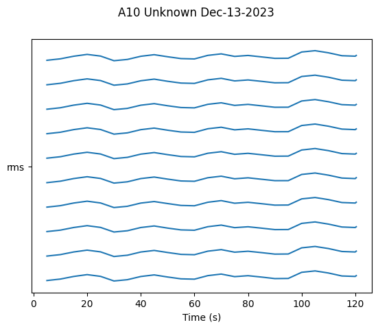
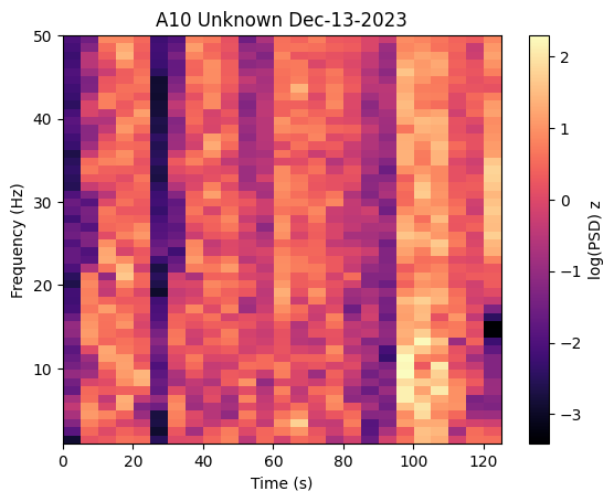
Use AnimalPlotter to visualize data over time from a single animal. Note: Do NOT aggregate time windows before plotting - the plotter needs the temporal data intact:

# Create plotter for single animal
ap = visualization.AnimalPlotter(war_filtered)

# Plot RMS over time
fig = ap.plot_linear_temporal(features=['rms'])
plt.show()

# Plot PSD band powers
fig = ap.plot_psd_spectrogram()
plt.show()

9. Aggregate Time Windows (Optional)

You can flatten all windows into a single value by averaging across time. This saves memory and gives you a summary statistic across an entire session.

Note: You should not aggregate before plotting time-series data with AnimalPlotter, as this removes the temporal information needed for over-time visualizations.

# Example: Aggregate for summary statistics
# Only do this if you need a single value per animal/session
war_aggregated = war_filtered.copy()
war_aggregated.aggregate_time_windows()

/home/runner/work/neurodent/neurodent/src/neurodent/visualization/results.py:2130: UserWarning: One or more channels do not match name aliases. Assuming alias from number in channel name.
  core.parse_chname_to_abbrev(x, assume_from_number=self.assume_from_number)
/home/runner/work/neurodent/neurodent/src/neurodent/visualization/results.py:4198: FutureWarning: DataFrameGroupBy.apply operated on the grouping columns. This behavior is deprecated, and in a future version of pandas the grouping columns will be excluded from the operation. Either pass `include_groups=False` to exclude the groupings or explicitly select the grouping columns after groupby to silence this warning.
  aggregated_df = result_grouped.apply(
/home/runner/work/neurodent/neurodent/src/neurodent/visualization/results.py:2130: UserWarning: One or more channels do not match name aliases. Assuming alias from number in channel name.
  core.parse_chname_to_abbrev(x, assume_from_number=self.assume_from_number)

Multi-Animal Comparison

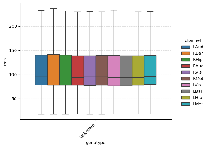
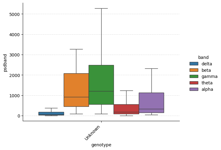
To compare across multiple animals, use ExperimentPlotter. Here we build a second WAR for animal F22 so we can compare the two:

# Build a WAR for a second animal (F22)
ao_f22 = visualization.AnimalOrganizer(
    pattern=[
        "../../.tests/integration/data/{animal}/*_ColMajor.bin",
        "../../.tests/integration/data/{animal}/*_Meta.csv",
    ],
    animal_id="F22",
    assume_from_number=True,
    lro_kwargs={
        "mode": "si",
        "extract_func": "../../tests/integration/readers.py:read_bin_csv_pair",
        "manual_datetimes": datetime(2023, 12, 12),
    },
)

war_f22 = ao_f22.compute_windowed_analysis(
    features=features, multiprocess_mode="serial"
)
war_f22_filtered = (
    war_f22
    .filter_logrms_range(z_range=3)
    .filter_high_rms(max_rms=500)
    .filter_low_rms(min_rms=10)
)

# Create ExperimentPlotter with both animals
wars = [war_filtered, war_f22_filtered]

ep = visualization.ExperimentPlotter(
    wars,
    features=features,
    exclude=['nspike', 'lognspike'],
    plot_order={'genotype': ['Unknown']},  # genotype is set via samples config; 'Unknown' is the default
)

# Categorical plot grouped by genotype
g = ep.plot_catplot(
    'rms',
    groupby='genotype',
    kind='box',
    catplot_params={'showfliers': False},
)
plt.show()

# PSD band powers grouped by genotype
g = ep.plot_catplot(
    'psdband',
    groupby='genotype',
    x='genotype',
    hue='band',
    kind='box',
    collapse_channels=True,
    catplot_params={'showfliers': False},
)
plt.show()

Processing rows:   0%|          | 0/94 [00:00<?, ?it/s]
Processing rows:   4%|▍         | 4/94 [00:00<00:02, 36.39it/s]
Processing rows:   9%|▊         | 8/94 [00:00<00:02, 37.23it/s]
Processing rows:  13%|█▎        | 12/94 [00:00<00:02, 37.68it/s]
Processing rows:  17%|█▋        | 16/94 [00:00<00:02, 37.81it/s]
Processing rows:  21%|██▏       | 20/94 [00:00<00:01, 37.81it/s]
Processing rows:  26%|██▌       | 24/94 [00:00<00:01, 37.89it/s]
Processing rows:  30%|██▉       | 28/94 [00:00<00:01, 37.92it/s]
Processing rows:  34%|███▍      | 32/94 [00:00<00:01, 37.95it/s]
Processing rows:  38%|███▊      | 36/94 [00:00<00:01, 37.90it/s]
Processing rows:  43%|████▎     | 40/94 [00:01<00:01, 37.80it/s]
Processing rows:  47%|████▋     | 44/94 [00:01<00:01, 37.89it/s]
Processing rows:  51%|█████     | 48/94 [00:01<00:01, 38.01it/s]
Processing rows:  55%|█████▌    | 52/94 [00:01<00:01, 37.91it/s]
Processing rows:  60%|█████▉    | 56/94 [00:01<00:01, 37.94it/s]
Processing rows:  64%|██████▍   | 60/94 [00:01<00:00, 37.90it/s]
Processing rows:  68%|██████▊   | 64/94 [00:01<00:00, 37.89it/s]
Processing rows:  72%|███████▏  | 68/94 [00:01<00:00, 37.93it/s]
Processing rows:  77%|███████▋  | 72/94 [00:01<00:00, 37.82it/s]
Processing rows:  81%|████████  | 76/94 [00:02<00:00, 37.80it/s]
Processing rows:  85%|████████▌ | 80/94 [00:02<00:00, 37.80it/s]
Processing rows:  89%|████████▉ | 84/94 [00:02<00:00, 37.81it/s]
Processing rows:  94%|█████████▎| 88/94 [00:02<00:00, 37.83it/s]
Processing rows:  98%|█████████▊| 92/94 [00:02<00:00, 37.88it/s]
/home/runner/work/neurodent/neurodent/src/neurodent/core/analyze_frag.py:423: RuntimeWarning: fmin=1.000 Hz corresponds to 1.440 < 5 cycles based on the epoch length 1.440 sec, need at least 5.000 sec epochs or fmin=3.472. Spectrum estimate will be unreliable.
  con = spectral_connectivity_epochs(
Processing rows: 100%|██████████| 94/94 [00:02<00:00, 38.03it/s]

WARNING:root:Missing LOF scores for F22_unknown! LOF computation may have failed or compute_bad_channels() was not called for this LRO.
WARNING:root:WARNING: 1 animalday(s) are missing LOF scores: ['F22_unknown']. Expected 1 but got 0. These sessions will be auto-populated with empty placeholders and excluded from LOF-based analysis.
/home/runner/work/neurodent/neurodent/src/neurodent/visualization/results.py:1384: UserWarning: WARNING: 1 animalday(s) are missing LOF scores: ['F22_unknown']. Expected 1 but got 0. These sessions will be auto-populated with empty placeholders and excluded from LOF-based analysis.
  warnings.warn(warning_msg)
WARNING:root:Added missing animalday to lof_scores_dict: F22 Unknown Dec-12-2023. This indicates LOF scores were not computed for this session. It will be excluded from LOF-based analysis.
/home/runner/work/neurodent/neurodent/src/neurodent/visualization/results.py:2130: UserWarning: One or more channels do not match name aliases. Assuming alias from number in channel name.
  core.parse_chname_to_abbrev(x, assume_from_number=self.assume_from_number)
/home/runner/work/neurodent/neurodent/src/neurodent/visualization/results.py:2130: UserWarning: One or more channels do not match name aliases. Assuming alias from number in channel name.
  core.parse_chname_to_abbrev(x, assume_from_number=self.assume_from_number)
/home/runner/work/neurodent/neurodent/src/neurodent/visualization/results.py:2130: UserWarning: One or more channels do not match name aliases. Assuming alias from number in channel name.
  core.parse_chname_to_abbrev(x, assume_from_number=self.assume_from_number)
/home/runner/work/neurodent/neurodent/src/neurodent/visualization/results.py:2130: UserWarning: One or more channels do not match name aliases. Assuming alias from number in channel name.
  core.parse_chname_to_abbrev(x, assume_from_number=self.assume_from_number)
/home/runner/work/neurodent/neurodent/src/neurodent/visualization/feature_utils.py:466: RuntimeWarning: Mean of empty slice
  return np.nanmean(vals, axis=channel_axes[0])

10. Save Results

You can save your WAR objects for later analysis:

import tempfile

# Use a temporary directory for demonstration purposes
with tempfile.TemporaryDirectory() as tmpdir:
    output_path = Path(tmpdir) / "A10"
    output_path.mkdir(parents=True, exist_ok=True)

    # Save WAR
    war_filtered.save_pickle_and_json(folder=output_path)
    print(f"WAR saved to {output_path}")

    # Load WAR
    war_loaded = visualization.WindowAnalysisResult.load_pickle_and_json(output_path)
    print(f"Loaded result for {war_loaded.animal_id}")

WAR saved to /tmp/tmp_vp7esfo/A10
Loaded result for A10

/home/runner/work/neurodent/neurodent/src/neurodent/visualization/results.py:2130: UserWarning: One or more channels do not match name aliases. Assuming alias from number in channel name.
  core.parse_chname_to_abbrev(x, assume_from_number=self.assume_from_number)

Summary

In this tutorial, you learned how to:

1. Import and configure Neurodent

2. Load EEG data using LongRecordingOrganizer (single path and DiscoveredFile)

3. Create an AnimalOrganizer for feature extraction

4. Compute windowed analysis features (WindowAnalysisResult)

5. Filter and clean data

6. (Optionally) Aggregate time windows for summary statistics

7. Visualize results using AnimalPlotter and ExperimentPlotter

8. Save and load results

Next Steps

• Data Loading Tutorial: Learn about loading different data formats

• Windowed Analysis Tutorial: Deep dive into feature extraction

• Visualization Tutorial: Advanced plotting techniques

• Spike Analysis Tutorial: Working with spike-sorted data